Community detection • nett

library(nett)

Spectral clustering

Let us sample a network from a DCSBM:

n = 1500
Ktru = 4
lambda = 15 # expected average degree
oir = 0.1
pri = 1:Ktru

set.seed(1234)
theta <- EnvStats::rpareto(n, 2/3, 3)
B = pp_conn(n, oir, lambda, pri=pri, theta)$B
z = sample(Ktru, n, replace=T, prob=pri) # randomly smaple "true community labels" 
A = sample_dcsbm(z, B, theta) # sample the adjacency matrix

We can apply the (Laplacian-based) regularized spectral clustering for community detection:

zh = spec_clust(A, K=4)

We can evaluate the performance by computing the normalized mutual information (NMI) to a true label vector:

compute_mutual_info(z, zh)
#> [1] 0.8459515

NMI is in \([0,1]\) and the closer to 1 it is the closer the mathc between the two labels.

Performance as a function of the expected degree

Let us now consider the effect of the expected average degree \(\lambda\) on the performance of spectral clustering.

Simple planted partition model

We first generate from a simple planted partition model, with connectivity matrix, \[B_1 \propto (1-\beta)I_{K}+ \beta\mathbf{1}\mathbf{1}^{T}\] where \(\beta\) is the out-in-ratio.

set.seed(1234)
nrep = 20
nlam = 12
lamvec = 10^seq(log10(1), log10(50), length.out = nlam)  # the vector of logarithmically spaced lambda
runs = expand.grid(rep = 1:nrep, lambda = lamvec)

res = do.call(rbind, lapply(1:nrow(runs), function(j) {
 lambda = runs[j,"lambda"]
 B = pp_conn(n, oir, lambda, pri=pri, theta)$B
 A = sample_dcsbm(z, B, theta)
 zh = spec_clust(A, K = Ktru) # defaults to tau = 0.25 for the  regularization parameter
 zh_noreg = spec_clust(A, K = Ktru, tau = 0)
 data.frame(rep = runs[j,"rep"], lambda = lambda, 
            nmi = compute_mutual_info(z, zh), nmi_noreg = compute_mutual_info(z, zh_noreg))
}))

agg_nmi = aggregate(res, by = list(res$lambda), FUN = mean)

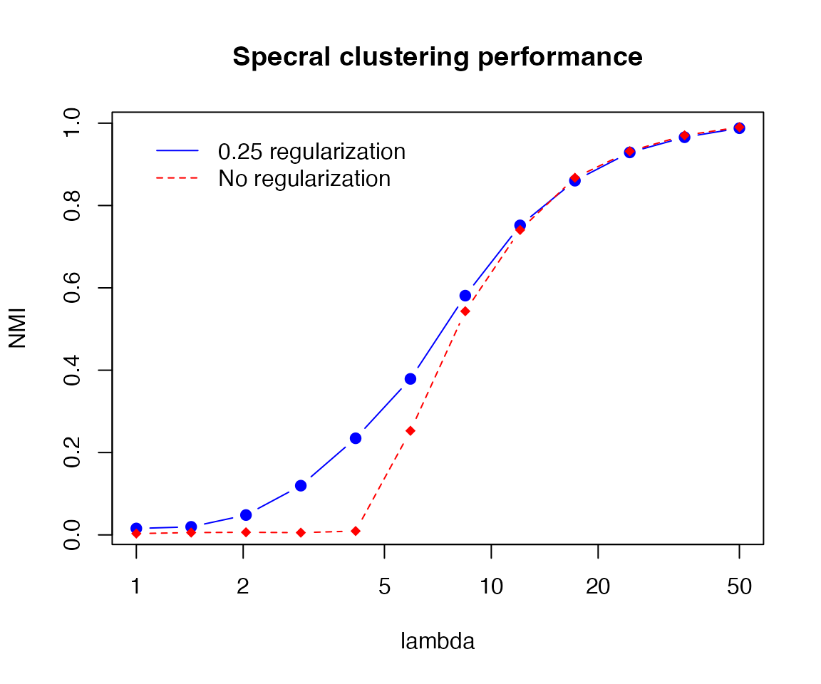
The resulting plot looks like this:

plot(agg_nmi$lambda, agg_nmi$nmi, log="x",
     type = "b", col = "blue", ylab = "NMI", xlab = "lambda", pch=19,
     main="Specral clustering performance")
lines(agg_nmi$lambda, agg_nmi$nmi_noreg, col="red", lty=2, pch=18, type = "b")
legend(1, 1, legend = c("0.25 regularization","No regularization"), 
       col = c("blue","red"), lty=1:2, box.lty=0)

This shows that increasing \(\lambda\) makes the community detection problem easier.

Randomly permuted connectivity matrix

Let us now generate the connectivity matrix randomly as follows \[B_2 \propto \gamma R + (1-\gamma) Q \] where

\(\gamma \in (0, 1)\),
\(R\) is a random symmetric permutation matrix (see function rsymperm()), and
\(Q\) a symmetric matrix with i.i.d. Unif\((0,1)\) entries on and above diagonal.

The function gen_rand_conn() generates such connectivity matrices.

set.seed(1234)
nrep = 20
nlam = 12
lamvec = 10^seq(log10(1), log10(200), length.out = nlam)  # the vector of logarithmically spaced lambda
runs = expand.grid(rep = 1:nrep, lambda = lamvec)

res = do.call(rbind, lapply(1:nrow(runs), function(j) {
 lambda = runs[j,"lambda"]
 B = gen_rand_conn(n, Ktru, lambda = lambda, gamma = 0.1, pri=pri)
 A = sample_dcsbm(z, B, theta)
 zh = spec_clust(A, K = Ktru) # defaults to tau = 0.25 for the  regularization parameter
 zh_noreg = spec_clust(A, K = Ktru, tau = 0)
 data.frame(rep = runs[j,"rep"], lambda = lambda, 
            nmi = compute_mutual_info(z, zh), nmi_noreg = compute_mutual_info(z, zh_noreg))
}))

agg_nmi = aggregate(res, by = list(res$lambda), FUN = mean)

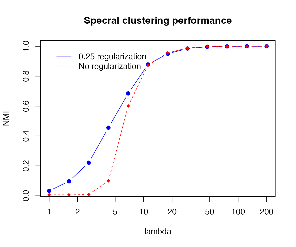
The resulting plot looks like the following:

plot(agg_nmi$lambda, agg_nmi$nmi, log="x",
     type = "b", col = "blue", ylab = "NMI", xlab = "lambda", pch=19,
     main="Specral clustering performance")
lines(agg_nmi$lambda, agg_nmi$nmi_noreg, col="red", lty=2, pch=18, type = "b")
legend(1, max(agg_nmi$nmi), legend = c("0.25 regularization","No regularization"), 
       col = c("blue","red"), lty=1:2, box.lty=0)